Simplified Phase-locked Loop in C

Update (14 Jan 2017) : I modified the loop filter design to be more consistent with common terminology in the literature.

If you read my last tutorial on writing a PLL in C and found it overly complex, this entry should hopefully clear some of that up. I received a lot of feedback on it and realize that I tend to make things unnecessarily complicated. Sorry.

So here is a super simple phase-locked loop in 50 lines of C. I've omitted the lengthy, boring, math (no more Laplace transforms!) and boiled down the PLL to its bare essentials. It's definitely a lot easier to understand, especially if you haven't had 3 semesters of electrical engineering courses to prepare you. I won't even include any equations (ok, maybe one).

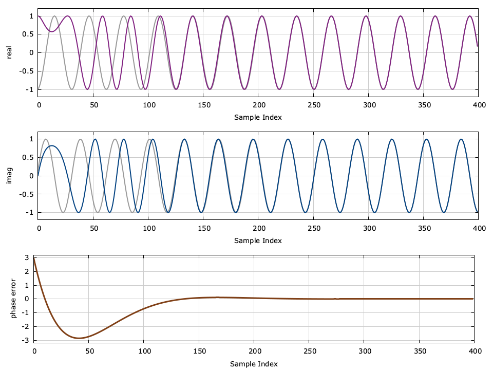
You can download a tarball of this example which includes all the source code here: liquid_pll_simple_example.tar.gz . Running the program should produce an image that looks like this:

Figure [pll_simple_example]. Simpler Phase-locked Loop Demonstration

Problem statement∞

I have an incoming complex sinusoid with an unknown but constant frequency and phase (and it's possibly noisy, but we won't add noise in our example). I want to track the phase of this input on a sample-by-sample basis. Basically I need to generate a new sinusoid (the output) that has the exact same phase and frequency as the input.

The concept of a PLL is simple:

1. Make a measurement of the phase error between the input signal and my output sinusoid.
2. Adjust my output signal's frequency and phase proportional to this phase error.
3. Repeat.

Sounds simple enough, right? The difficulty is knowing precisely how to execute step 2 to get the output to converge and not blow up (that's where all that math from the previous post came in). There's a simple trick to you can use to get really good performance:

• Define a variable \(\alpha\) as the the proportion of the phase error we will apply to adjust our output phase . Note that \(\alpha\) is proportional to the loop filter bandwidth and so it should be relatively small (e.g. 0.05 or so).
• Define a new variable \(\beta = \alpha^2/2\) . This value will be the proportion of the phase error we will apply to adjust our output frequency .

Source Code Breakdown∞

So here's the program in 50 lines (as promised):

// pll_simple_example.c : simulation of a phase-locked loop in 50 lines
// [update] 14 Jan. 2017: updated loop filter to be consistent with literature
#include <stdio.h>
#include <stdlib.h>
#include <complex.h>
#include <math.h>

int main() {
    // parameters and simulation options
    float        phase_in      =  3.0f;    // carrier phase offset
    float        frequency_in  = -0.20;    // carrier frequency offset
    float        alpha         =  0.05f;   // phase adjustment factor
    unsigned int n             =  400;     // number of samples

    // initialize states
    float beta          = 0.5*alpha*alpha; // frequency adjustment factor
    float phase_out     = 0.0f;            // output signal phase
    float frequency_out = 0.0f;            // output signal frequency

    // print line legend to standard output
    printf("# %6s %12s %12s %12s %12s %12s\n",
           "index", "real(in)", "imag(in)", "real(out)", "imag(out)", "error");

    // run basic simulation
    int i;
    for (i=0; i<n; i++) {
        // compute input and output signals
        float complex signal_in  = cexpf(_Complex_I * phase_in);
        float complex signal_out = cexpf(_Complex_I * phase_out);

        // compute phase error estimate
        float phase_error = cargf( signal_in * conjf(signal_out) );

        // print results to standard output for plotting
        printf("  %6u %12.8f %12.8f %12.8f %12.8f %12.8f\n",
                  i,
                  crealf(signal_in),  cimagf(signal_in),
                  crealf(signal_out), cimagf(signal_out),
                  phase_error);

        // apply loop filter and correct output phase and frequency
        phase_out     += alpha * phase_error;    // adjust phase
        frequency_out +=  beta * phase_error;    // adjust frequency

        // increment input and output phase values
        phase_in  += frequency_in;
        phase_out += frequency_out;
    }
    return 0;
}

Compiling and running the program will produce an output data file should look similar to this:

#  index     real(in)     imag(in)    real(out)    imag(out)        error
       0  -0.98999250   0.14112000   1.00000000   0.00000000   3.00000000
       1  -0.94222230   0.33498821   0.98820370   0.15314497   2.64625001
       2  -0.85688871   0.51550144   0.95734698   0.28894085   2.30687952
       3  -0.73739362   0.67546326   0.91373789   0.40630421   1.98159420
       4  -0.58850098   0.80849653   0.86285567   0.50545037   1.67009592
       5  -0.41614661   0.90929753   0.80925429   0.58745849   1.37208498
       6  -0.22720182   0.97384769   0.75657302   0.65390921   1.08725977
     ...
     394   0.92037261  -0.39104259   0.92032784  -0.39114791   0.00011444
     395   0.82433999  -0.56609505   0.82427084  -0.56619567   0.00012207
     396   0.69544452  -0.71857977   0.69535130  -0.71867001   0.00012973
     397   0.53882474  -0.84241790   0.53870904  -0.84249187   0.00013733
     398   0.36072436  -0.93267244   0.36058915  -0.93272477   0.00014499
     399   0.16824348  -0.98574549   0.16809307  -0.98577112   0.00015259

Ideally when the simulation is finished, the input phase and output phase should be equal (modulo \(2\pi\) ) and so should the input/output frequencies. From the results we can make a few observations:

• The phase error at the first step is exactly 3 radians, the input phase.
• The magnitude of the error drops, on average, with each step.
• The signals are nearly identical by the last iteration.

So why didn't I present this simpler, more elegant PLL design in my previous post ? Chalk it up to being in academia too long.