Windowing Functions

This section describes the various windowing functions in the math module. These windowing functions are useful for spectral approximation as they are compact in both the time and frequency domains. See hamming(), Hamming window for more details.

Interfaces

hamming(), Hamming window

The function hamming computes the \(n^{th}\) of \(N\) indices of the Hamming window:

(32)\[w(n) = 0.53836 - 0.46164 \cos\left( 2 \pi n / (N-1) \right)\]

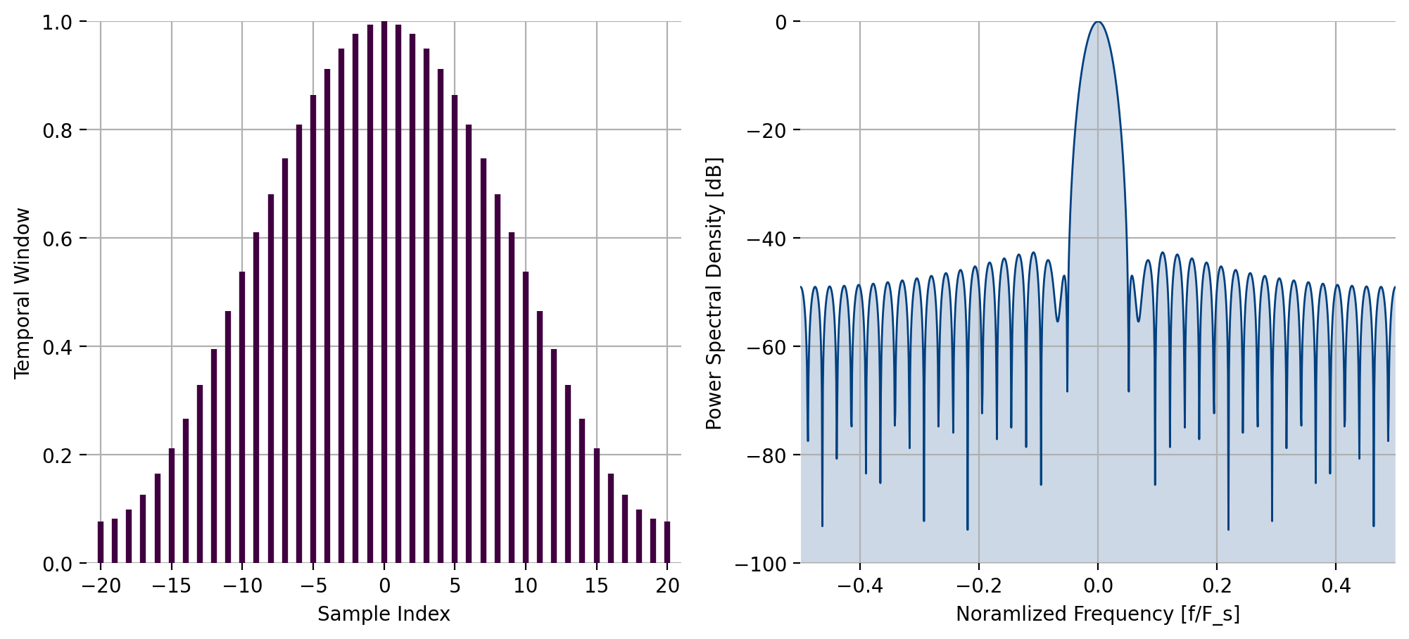
Figure 19 Hamming window response

hann(), Hann window

The function hann computes the \(n^{th}\) of \(N\) indices of the Hann window:

(33)\[w(n) = 0.5 - 0.5 \cos\left( 2 \pi n / (N-1) \right)\]

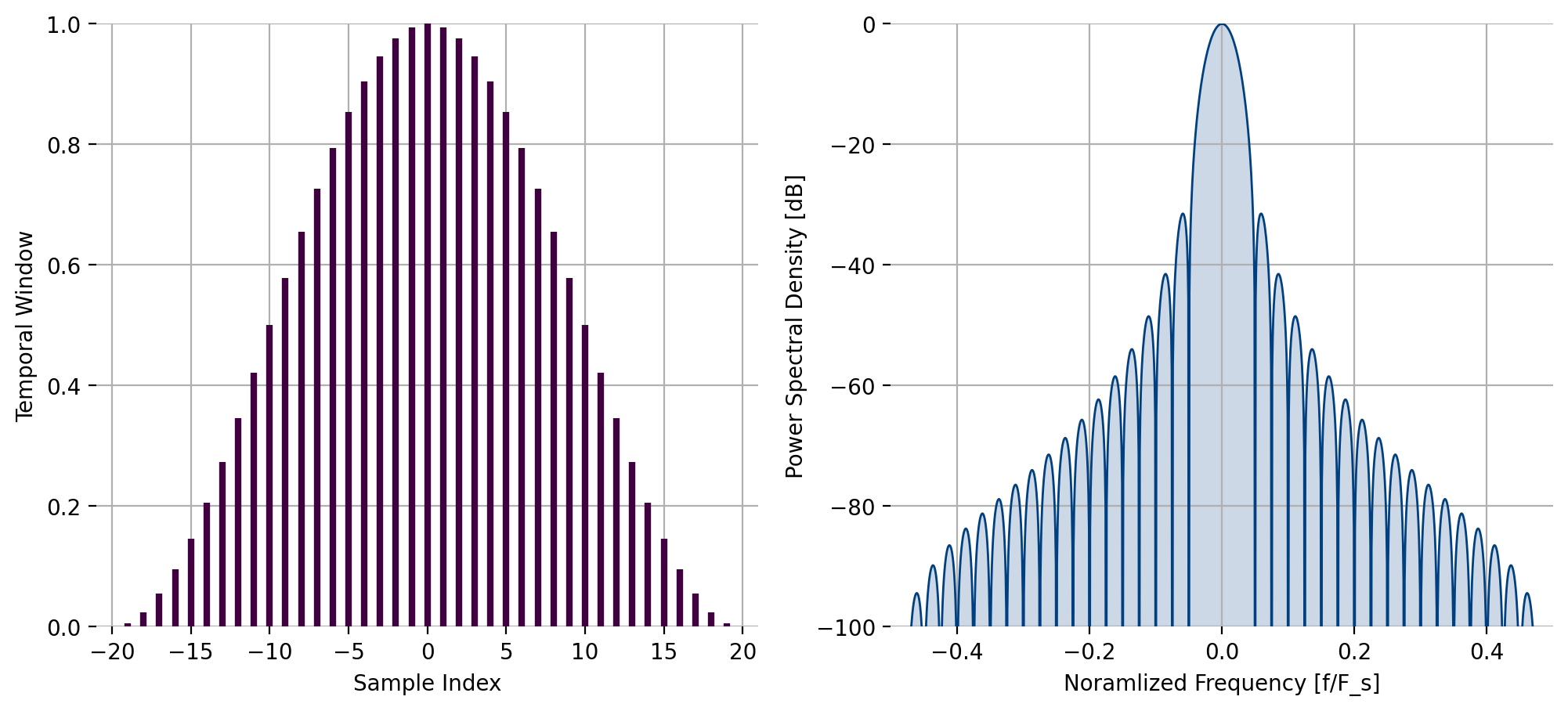
Figure 20 Hann window response

blackmanharris(), Blackman-harris window

The function blackmanharris computes the \(n^{th}\) of \(N\) indices of the Blackman-harris window:

(34)\[w(n) = \sum_{k=0}^{3} { a_k \cos\left( 2 \pi k n / (N-1)\right) }\]

where \(a_0 = 0.35875\), \(a_1 = -0.48829\), \(a_2 = 0.14128\), and \(a_3 = -0.01168\).

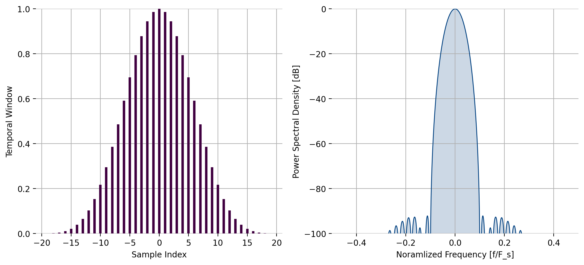
Figure 21 Blackman-harris window response

blackmanharris7(), 7th-order Blackman-harris Window

The function blackmanharris7 computes the \(n^{th}\) of \(N\) indices of the 7:math:^{th}-order Blackman-harris window:

(35)\[w(n) = \sum_{k=0}^{3} { a_k \cos\left( 2 \pi k n / (N-1)\right) }\]

where \(a_0 = 0.27105\), \(a_1 = 0.43329\), \(a_2 = 0.21812\), \(a_3 = 0.06592\), \(a_4 = 0.01081\), \(a_5 = 0.00077\), and \(a_6 = 0.00001\).

Notice that the side-lobes have been suppressed below 100 dB at the expense of a wider main lobe.

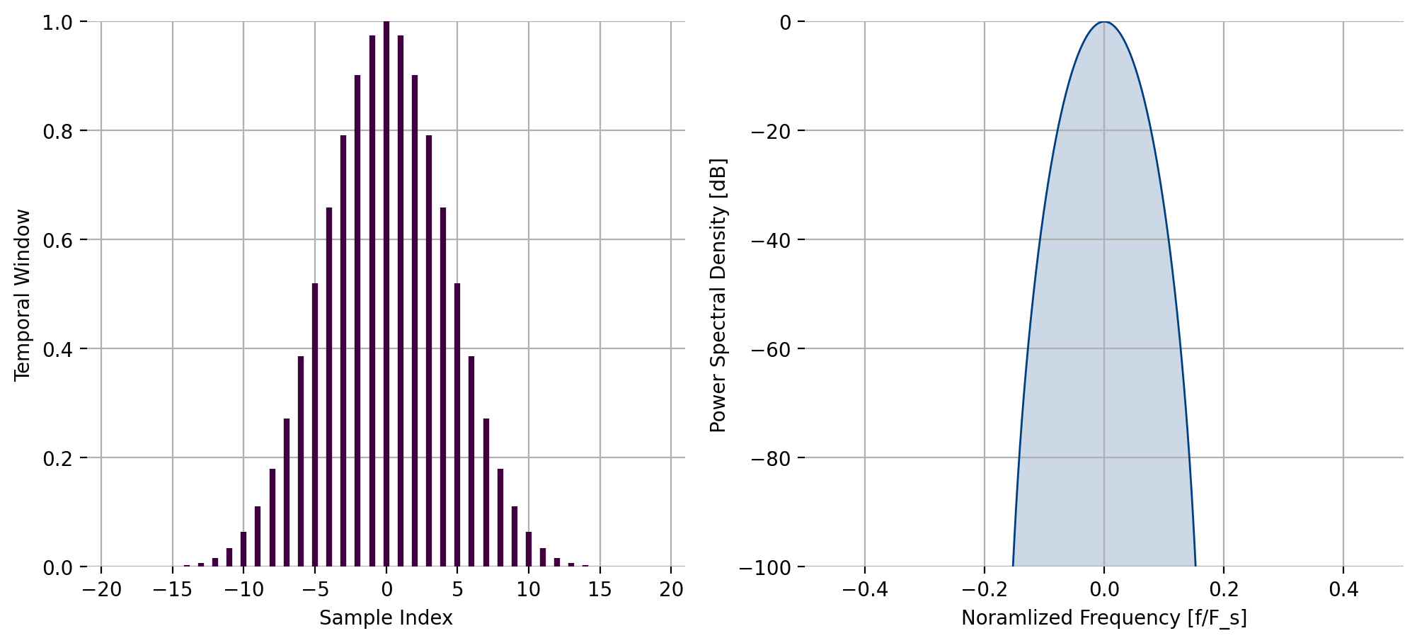
Figure 22 Blackman-harris (7) window response

flattop(), Flat-top Window

The function flattop computes the \(n^{th}\) of \(N\) indices of the Flat-top window:

(36)\[w(n;N) = 1 - 1.93 \cos\left( \frac{n}{N}\right) + 1.29 \cos\left(2\frac{n}{N}\right) - 0.388\cos\left(3\frac{n}{N}\right) + 0.028\cos\left(4\frac{n}{N}\right)\]

Notice that the response looks similar to a low-pass non-recursive [filter design][/doc/firdes/], allows the window to have negative values, and has a peak much greater than one.

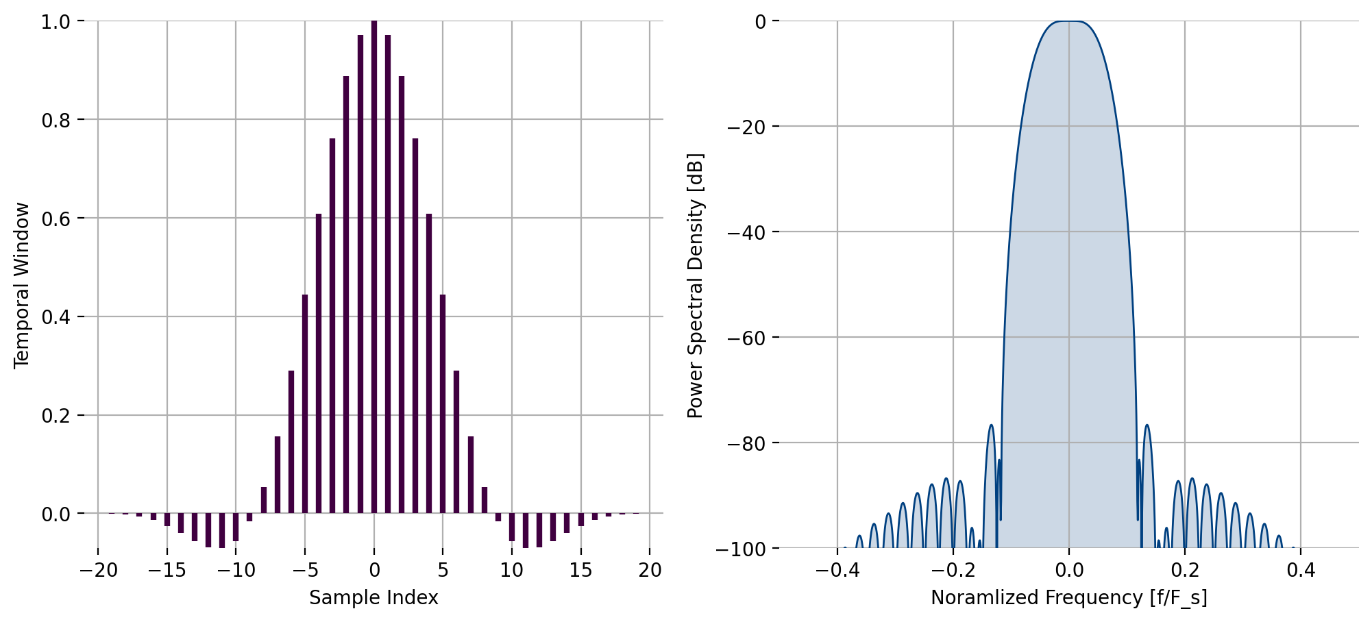
Figure 23 Flat top window response

triangular(), Triangular window

The function triangular computes the \(n^{th}\) of \(N\) indices of the triangular window:

(37)\[w(n;N) = 1 - \left| \frac{n - \frac{N-1}{2} }{\frac{L}{2}}\right|\]

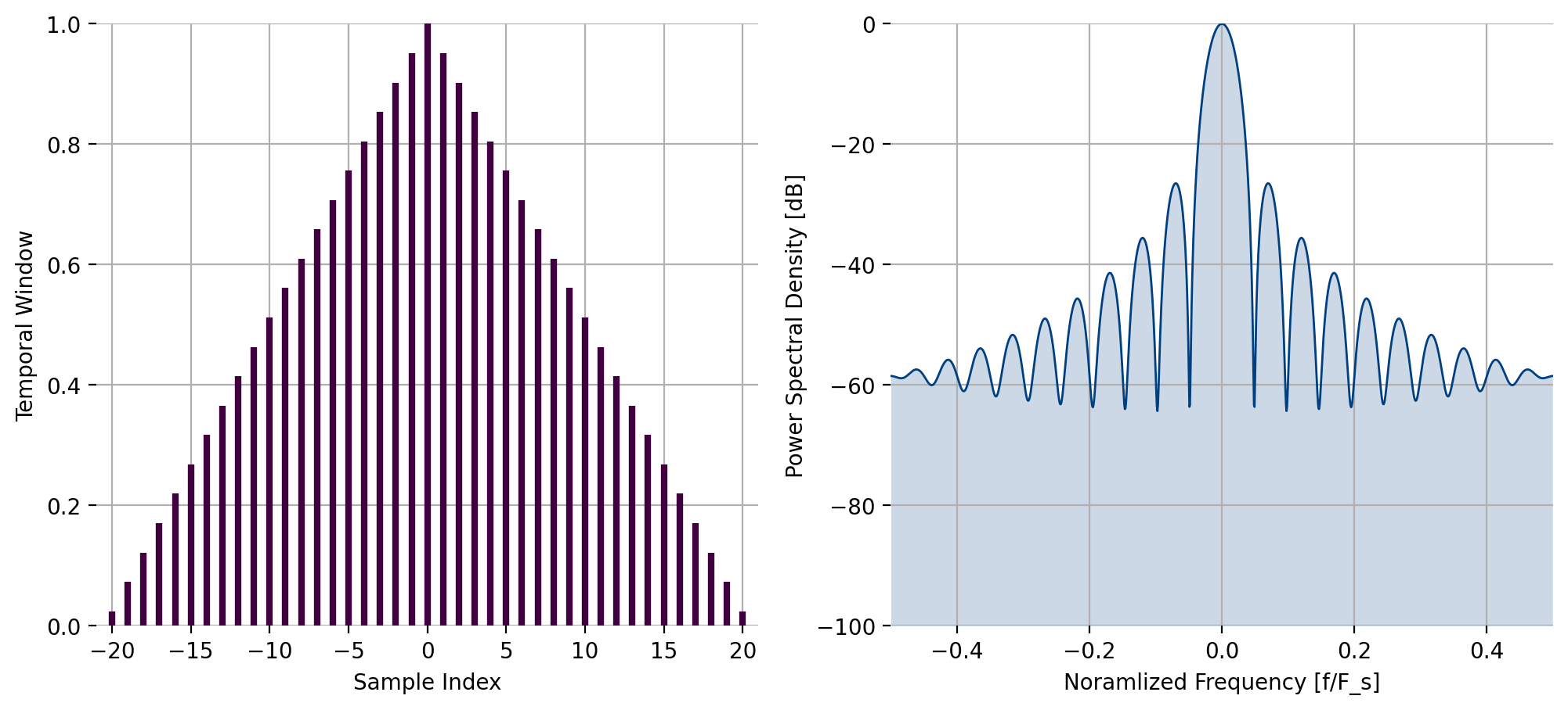
Figure 24 Triangular window response

kaiser(), Kaiser-Bessel window

The function kaiser computes the \(n^{th}\) of \(N\) indices of the Kaiser-\(\beta\) window with a shape parameter \(\beta\):

(38)\[w(n,\beta) = \frac{ I_0\left(\pi\beta\sqrt{1-\left(\frac{n}{N/2}\right)^2}\right) }{ I_0\left(\pi\beta\right) }\]

where \(I_\nu(z)\) is the modified Bessel function of the first kind of order \(\nu\), and \(\beta\) is a parameter controlling the width of the window and its stop-band attenuation. In liquid, \(I_0(z)\) is computed using liquid_besseli0f() (see [section-math-transcendentals]). A fractional sample offset \(\Delta t\) can be introduced by substituting \(\frac{n}{N/2}\) with \(\frac{n+\Delta t}{N/2}\) in [eqn-math-window-kaiser].

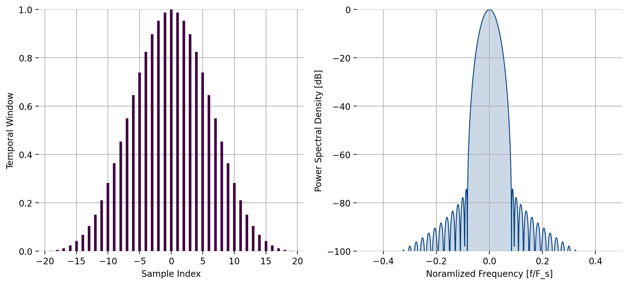
Figure 25 Kaiser window response, \(\beta = 10\)

liquid_kbd_window(), Kaiser-Bessel derived window

The function liquid_kbd_window computes the \(n\)-point Kaiser-Bessel derived window with a shape parameter \(\beta\) storing the result in the \(n\)-point array w. The length of the window must be even.

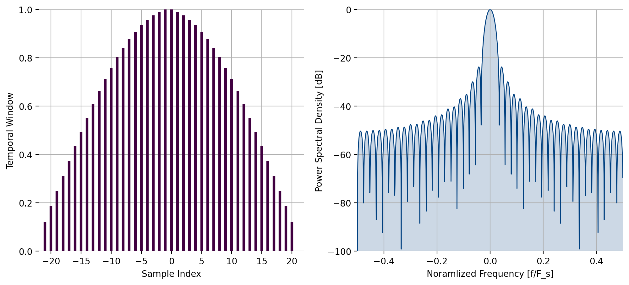
Figure 26 Kaiser-Besssel derived window response, \(beta = 10\)

liquid_rcostaper_windowf(), Raised-Cosine Tapering Window

The function liquid_rcostaper_windowf computes the \(n^{th}\) of \(N\) indices of the raised-cosine tapering window with t samples on the front and tail used for tapering.

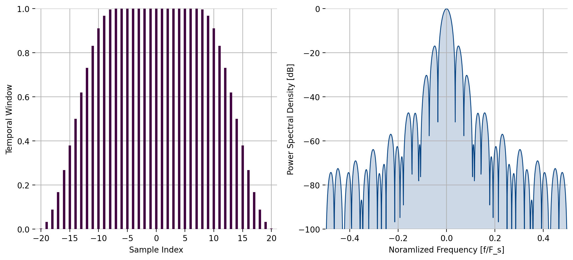
Figure 27 Raised-Cosine taper window response